Tutorial 03 - Introduction to neural data types
Goals
- Become aware of the processing steps typically applied to raw data acquired with a Neuralynx system
- Learn the data types used for neural data analysis
- Use the loading functions for all these files
Data processing
Renaming
The naming convention in our lab is: R###-YYYY-MM-DD-filetype.extension
By default, Neuralynx will name files filetype.extension, so the ratID and date need to be added as a prefix. This can be done with a script, just be careful to double-check that your script only renames the files.
Manual annotation
Some common features that are manually annotated are: - experimenter name - subject ID - session ID - experiment time blocks
These are stored for easy access in an info.py file within your
project folder.
Spike sorting
Spike sorting is the process of automated and manual detection of individual units from a tetrode or probe recording. See Module08 for details.
Data files overview
A typical recording session from a Neuralynx system contains:
- ‘’.ncs’’ (“Neuralynx Continuously Sampled”) files typically contain local field potentials (LFPs) sampled at 2kHz and filtered between 1 and 475 Hz.
- ‘’.t’ or ‘’._t’’ (“Tetrode”) files, which are generated by MClust from the raw ‘’.ntt’’ (“Neuralynx TeTrode”) files contains a set of times from individual putative neurons.
- ‘’.nvt’’ (“Neuralynx Video Tracking”) file contains the location of the rat as tracked by an overhead camera, typically sampled at 30 Hz.
- ‘’.nev’’ (“Neuralynx EVents”) file contains timestamps and labels of events
- ‘’info.py’’ file contains experimenter-provided information that describes this data set.
Nept data types
Documentation for all the data types we use in Nept can be found here. But we’ll also briefly describe them in this module.
AnalogSignal
Genrally, data acquisition systems work by sampling some quantity of
interest, so often only periodically measurements are taken. A sampled
signal is essentially a list of values (data points), taken at specific
times. Thus, what we need to fully describe such a signal is two arrays
of the same length: one with the timestamps and the other with the
corresponding data. For this, we use an AnalogSignal, which has
time and data fields.
LocalFieldPotential
A LocalFieldPotential is a subclass of AnalogSignal.
Position
A Position is a subclass of AnalogSignal, with some unique
methods that are useful when dealing with positions. This includes
computing the distance between two positions, or computing the
speed of the position.
Epoch
Epochs describe occurrences that have start and stop times, such as a trial of an experiment or the presence of a cue (e.g. a light or a tone).
SpikeTrain
Much of neuroscience analyses attributes particular significance to action potentials, or “spikes”, which are typically understood as all-or-none events that occur at a specific point in time. It is not necessary to state all the times at which there was no spike to describe a train of spikes; it suffices to maintain a list of those times (known as “timestamps”) at which a spike was emitted.
Loading real data
In [1]:
# import necessary packages
%matplotlib inline
import os
import sys
import numpy as np
import nept
import matplotlib.pyplot as plt

# Define where your data folder is located
data_path = os.path.join(os.path.abspath('.'), 'data')
data_folder = os.path.join(data_path, 'R016-2012-10-03')
In [2]:
# Load the info file, which contains experiment-specific information
sys.path.append(data_folder)
import r016d3 as info
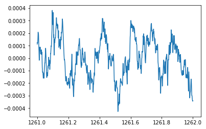
In [3]:
# Load LFP (.ncs) from rat ventral striatum (same as Module01)
lfp = nept.load_lfp(os.path.join(data_folder, info.lfp_theta_filename))

# Slice the LFP to our time of interest
start = 1261
stop = 1262
sliced_lfp = lfp.time_slice(start, stop)

# Plot the sliced LFP
plt.plot(sliced_lfp.time, sliced_lfp.data)
plt.show()
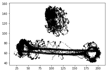
In [4]:
# Load position (.nvt) from this experiment
position = nept.load_position(os.path.join(data_folder, info.position_filename),
                              info.pxl_to_cm)

# Plot the position
plt.plot(position.x, position.y, 'k.', ms=1)
plt.show()
In [5]:
# Load events (.nev) from this experiment
events = nept.load_events(os.path.join(data_folder, info.event_filename),
                          info.event_labels)

# Print what events we're working with
print(events.keys())
dict_keys(['cue3', 'pellet2', 'cue2or4', 'feeder1', 'pellet4', 'feeder0', 'start', 'cue5', 'pellet3', 'pellet5', 'pellet1', 'cue1or5', 'cue1'])
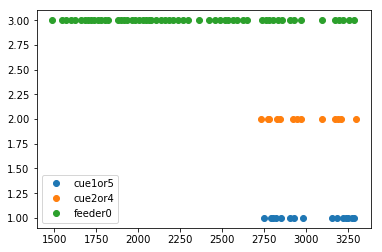
In [6]:
# Plot the events
plt.plot(events['cue1or5'], np.ones(len(events['cue1or5'])), 'o')
plt.plot(events['cue2or4'], np.ones(len(events['cue2or4']))+1, 'o')
plt.plot(events['feeder0'], np.ones(len(events['feeder0']))+2, 'o')
plt.legend(['cue1or5', 'cue2or4', 'feeder0'])
plt.show()
In [7]:
# Load spikes (.t and ._t) from this experiment
spikes = nept.load_spikes(data_folder)

# Plot the spikes
for idx, spiketrain in enumerate(spikes):
    plt.plot(spiketrain.time, np.ones(len(spiketrain.time))+idx, '|')
plt.show()

# Print the number of spikes emitted from each neuron
for idx, spiketrain in enumerate(spikes):
    print('Neuron', idx+1, 'has', len(spiketrain.time), 'spikes')
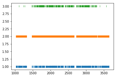
Neuron 1 has 4536 spikes
Neuron 2 has 32457 spikes
Neuron 3 has 4257 spikes
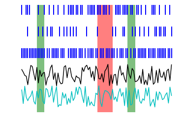
Summary
Together, these three types of data can describe most data sets encountered in neuroscience. Putting them together in a simple visualization might look something like this, with LFP in black, position in cyan, epochs in red and green, and spikes in blue:
In [8]:
import random

# Construct LFP
time = np.arange(100)
data = np.array(random.sample(range(100), 100)) / 100

toy_lfp = nept.LocalFieldPotential(data, time)

# Plot the LFP
plt.plot(toy_lfp.time, toy_lfp.data, 'k')

# Construct 1D position
time = np.arange(100)
x = np.array(random.sample(range(100), 100)) / -100

toy_position = nept.Position(x, time)

# Plot the position
plt.plot(toy_position.time, toy_position.x, 'c')

# Construct some epochs, which might be something like a light cue and a sound cue
toy_light = nept.Epoch(np.array([[10, 15],
                                 [70, 75]]))

toy_sound = nept.Epoch(np.array([[50, 60]]))

# Plot the epochs
for light_start, light_stop in zip(toy_light.starts, toy_light.stops):
    plt.axvspan(light_start, light_stop, color='g', alpha=0.5, lw=0)

for sound_start, sound_stop in zip(toy_sound.starts, toy_sound.stops):
    plt.axvspan(sound_start, sound_stop, color='r', alpha=0.5, lw=0)

# Construct some spikes
toy_spikes = [nept.SpikeTrain(np.array(random.sample(range(100), 80))),
              nept.SpikeTrain(np.array(random.sample(range(100), 30))),
              nept.SpikeTrain(np.array(random.sample(range(100), 50)))]

# Plot the spikes
for idx, spiketrain in enumerate(toy_spikes):
    plt.plot(spiketrain.time, np.ones(len(spiketrain.time))+idx+0.5, '|', color='b', ms=20, mew=2)

# Turn off axis
plt.axis('off')

plt.show()
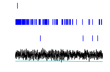
In [9]:
# With real data, this might look something more like this:

# Define our time of interest
start = 1240
stop = 1250

# Slice the LFP to our time of interest
sliced_lfp = lfp.time_slice(start, stop)

# Plot the LFP
plt.plot(sliced_lfp.time, sliced_lfp.data*1000, 'k')

# Slice the position to our time of interest
sliced_position = position.time_slice(start, stop)

# Plot the position
plt.plot(sliced_position.time, sliced_position.x*-0.001-0.3, 'c')

# Let's only work with one event, our event of interest
event_of_interest = events['pellet1']

# Slice our event to the time of interest
sliced_event = event_of_interest[(start < event_of_interest) & (event_of_interest < stop)]
if len(sliced_event) % 2 != 0: # remove last sample if odd number of events
    sliced_event = sliced_event[:-1]

# For visualization purposes, let's say this event was present for a certain amount of time
# and can be represented as an epoch, with a start and a stop
event_epoch = nept.Epoch([sliced_event[::2], sliced_event[1::2]])

# Plot the epoch
for epoch_start, epoch_stop in zip(event_epoch.starts, event_epoch.stops):
    plt.axvspan(epoch_start, epoch_stop, color='r', alpha=0.5, lw=0)

# Slice our spikes to the time of interest
sliced_spikes = [spiketrain.time_slice(start, stop) for spiketrain in spikes]

# Plot the spikes
for idx, spiketrain in enumerate(sliced_spikes):
    plt.plot(spiketrain.time, np.ones(len(spiketrain.time))+idx, '|', color='b', ms=20, mew=2)

# Turn off axis
plt.axis('off')

plt.show()
Real world examples
Here are two examples that illustrate some simple operations. You should run them and make sure you understand how the raw data is transformed. For this, we will use a more involved data set R042-2013-08-18, which has recordings from hippocampal CA1 neurons.
In [10]:
# import necessary packages
%matplotlib inline
import os
import sys
import numpy as np
import nept
import matplotlib.pyplot as plt
import scipy.stats

# define where your data folder is located
data_path = os.path.join(os.path.abspath('.'), 'data')
data_folder = os.path.join(data_path, 'R042-2013-08-18')
In [11]:
# load the info file, which contains experiment-specific information
sys.path.append(data_folder)
import r042d3 as info
In [12]:
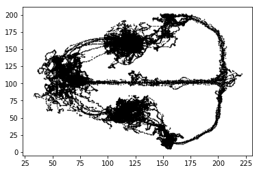
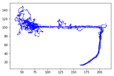
# Load position (.nvt) from this experiment
position = nept.load_position(os.path.join(data_folder, info.position_filename), info.pxl_to_cm)

# Plot the position
plt.plot(position.x, position.y, 'k.', ms=1)
plt.show()
In [13]:
left = position.time_slice(info.experiment_times['left_trials'].starts,
                           info.experiment_times['left_trials'].stops)

plt.plot(left.x, left.y, 'b.', ms=1)
plt.show()
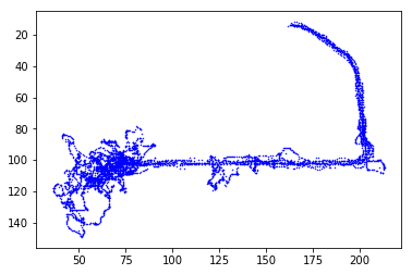
In [14]:
# This looks like right trials because the camera reverses the image.
# We can fix this by reversing the y_axis

plt.plot(left.x, left.y, 'b.', ms=1)
plt.gca().invert_yaxis()
plt.show()
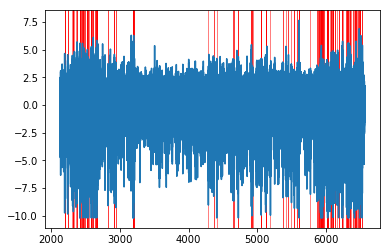
Now let’s look at how these data types can work together to detect potential artifacts in the LFP.
In [15]:
# Load LFP with good sharp-wave ripples
lfp_swr = nept.load_lfp(os.path.join(data_folder, info.lfp_swr_filename))

# Normalize the LFP
lfp_norm = nept.LocalFieldPotential(scipy.stats.zscore(lfp_swr.data), lfp_swr.time)

# Detect possible artifacts, save as epochs
thresh = -8
below_thresh = np.squeeze(lfp_norm.data < thresh)
below_thresh = np.hstack([[False], below_thresh, [False]]) # pad start and end to properly compute the diff

get_diff = np.diff(below_thresh.astype(int))

artifact_starts = lfp_norm.time[np.where(get_diff == 1)[0]]
artifact_stops = lfp_norm.time[np.where(get_diff == -1)[0]]

artifacts = nept.Epoch([artifact_starts, artifact_stops])

# Plot the LFP and artifact epochs
plt.plot(lfp_norm.time, lfp_norm.data)

for epoch_start, epoch_stop in zip(artifacts.starts, artifacts.stops):
    plt.axvspan(epoch_start, epoch_stop, color='r', alpha=0.5, lw=1)

plt.show()